
An EDS system — energy-dispersive X-ray spectroscopy — sits on a scanning or a transmission electron microscope and does one thing very well: it sorts X-ray photons by energy. The incident beam knocks an inner-shell electron out of a sample atom; an outer electron falls into the vacancy, and the energy difference leaves the atom as a characteristic X-ray. A silicon drift detector (SDD) measures each photon and bins it by energy, so the resulting spectrum carries energy across the horizontal axis and counts up the vertical one.
Reading a spectrum takes two steps. Peak positions say which elements are present. Turning peaks into concentrations is harder: the net intensity left after the continuous background is removed has to be measured against standards and corrected for the three matrix effects — atomic number, absorption and fluorescence. Line energy itself falls with atomic number within a given shell, which is why the K lines of the lightest elements sit at the very bottom of the spectrum.
In materials work, “light elements” means boron through fluorine — atomic numbers 5 to 9. Only their K lines are available, and all of them fall below 1 keV: B Kα at about 183.5 eV, then C, N and O Kα at about 0.28, 0.39 and 0.53 keV.
That region is crowded. The L lines of the transition metals and the M lines of still heavier elements land in the same window, and the continuous background — shaped by absorption edges and by the detector's own response — is at its most complicated below 2 keV.
A Cr₂N precipitate in high-nitrogen stainless steel shows what this costs in practice. STEM-EDS has no trouble demonstrating that Cr is enriched in the precipitate. The nitrogen map, by contrast, has a signal-to-noise ratio of about 1.03, and the nitrogen-depleted zones flanking the precipitate simply cannot be picked out of the raw data.
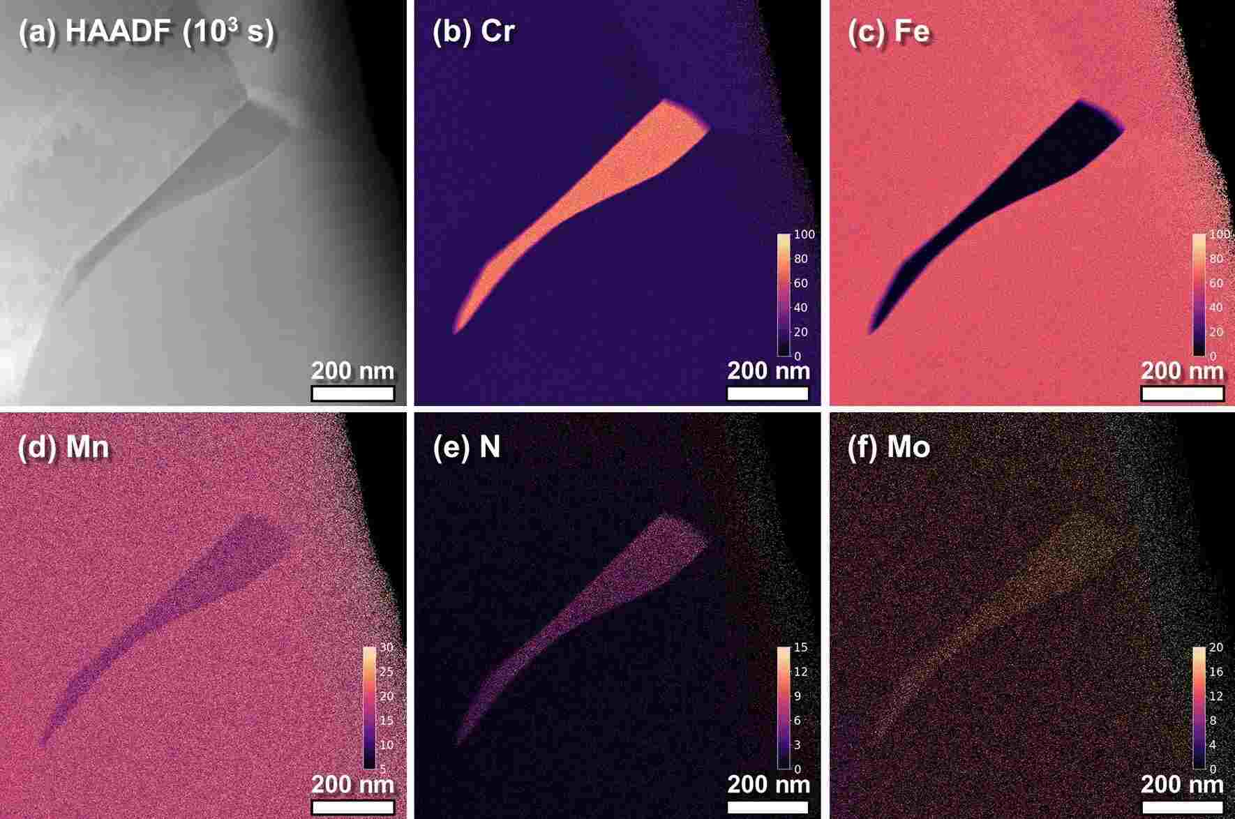
Figure 1. HAADF-STEM image of a Cr₂N precipitate in high-nitrogen stainless steel aged at 900 °C for 10³ s, together with EDS elemental maps of Cr, Fe, Mn, N and Mo. DOI: 10.1038/s41598-020-70674-y
Part of the explanation is that light atoms are stingy with characteristic X-rays, and the lighter the atom, the stingier they get. Hydrogen and helium produce nothing usable at all.
Lithium is the extreme case. With only 1s and 2s electrons, its 2s → 1s transition falls foul of the dipole selection rule; once lithium bonds ionically or covalently the outer electrons are drawn away, and the K-shell vacancy has nothing left to fall into it. Only metallic lithium, or a bonding state with some p character, yields the faint Li Kα line at about 52 eV.
Detectors built for low-energy X-rays can still find it. A windowless system running at 3.5 keV picks out the Li peak in the metal and in some lithium compounds — provided the analyst also rules out lines sharing the region, such as Al Lα at 72 eV and Si Lα at 92 eV.
Everything starts with the way a vacancy relaxes. Given an inner-shell hole, an atom has two options: emit a characteristic X-ray, or hand the energy to another outer electron and eject it as an Auger electron. The probability of taking the X-ray route is the fluorescence yield ωK, and it collapses as the atomic number falls — which is precisely why the Auger channel dominates for light elements.
Krause's compilation of K-shell data gives ωK of about 0.0028 for C, 0.0083 for O, 0.050 for Si and 0.340 for Fe. Create 1000 K-shell vacancies in carbon and roughly 3 X-ray photons come out; do the same in iron and roughly 340 do.
A low yield means few counts for a given beam current and acquisition time, and few counts mean large statistical scatter. More current or a longer dwell will buy counts, but it buys dose with them: the carbon contamination layer thickens and beam damage accumulates.
Then the photon has to escape. Low-energy X-rays are absorbed far more strongly than high-energy ones, so the deeper the electrons penetrate, the longer the path to the surface and the larger the absorption correction — and the uncertainty that goes with it. Under conventional conditions at 10 keV and above, NIST found that peaks below 1.5 keV quantified with more bias than high-energy peaks, and that the bias grew as the voltage rose.
The entrance window is the last obstacle. A conventional windowed system works mainly above C Kα; below that, photons are either blocked outright or arrive with a poor signal-to-noise ratio, and windowed detectors generally need nanoampere currents and more than 5 keV to collect enough counts.
Windowless operation changes those numbers. An SDD is already more sensitive below 1 keV than the old Si(Li) detectors, and removing the window eliminates film absorption and sharpens low-energy amplification, so X-rays below C Kα can be gathered at a few hundred picoamperes and under 5 keV.
Resolution is the first problem. A windowless SDD reaches about 47.5 eV at C Kα and 58.8 eV at F Kα, while the gap between a light-element K line and a neighbouring L line is often only tens of eV, a little over a hundred at most. Ti L sits near 0.45 keV and the Cr L lines near 0.50 and 0.57 keV, right among N Kα at 0.39 keV and O Kα at 0.53 keV.
Fitting can disentangle some of this. NIST measured Cr₂N at 10 keV against pure Cr and Si₃N₄ references by multiple linear least squares and obtained a nitrogen atomic fraction of 0.350 against an ideal 0.333 — a relative deviation of +5.1%, the worst of the nitrides tested, where TiN came in at +2.0%.
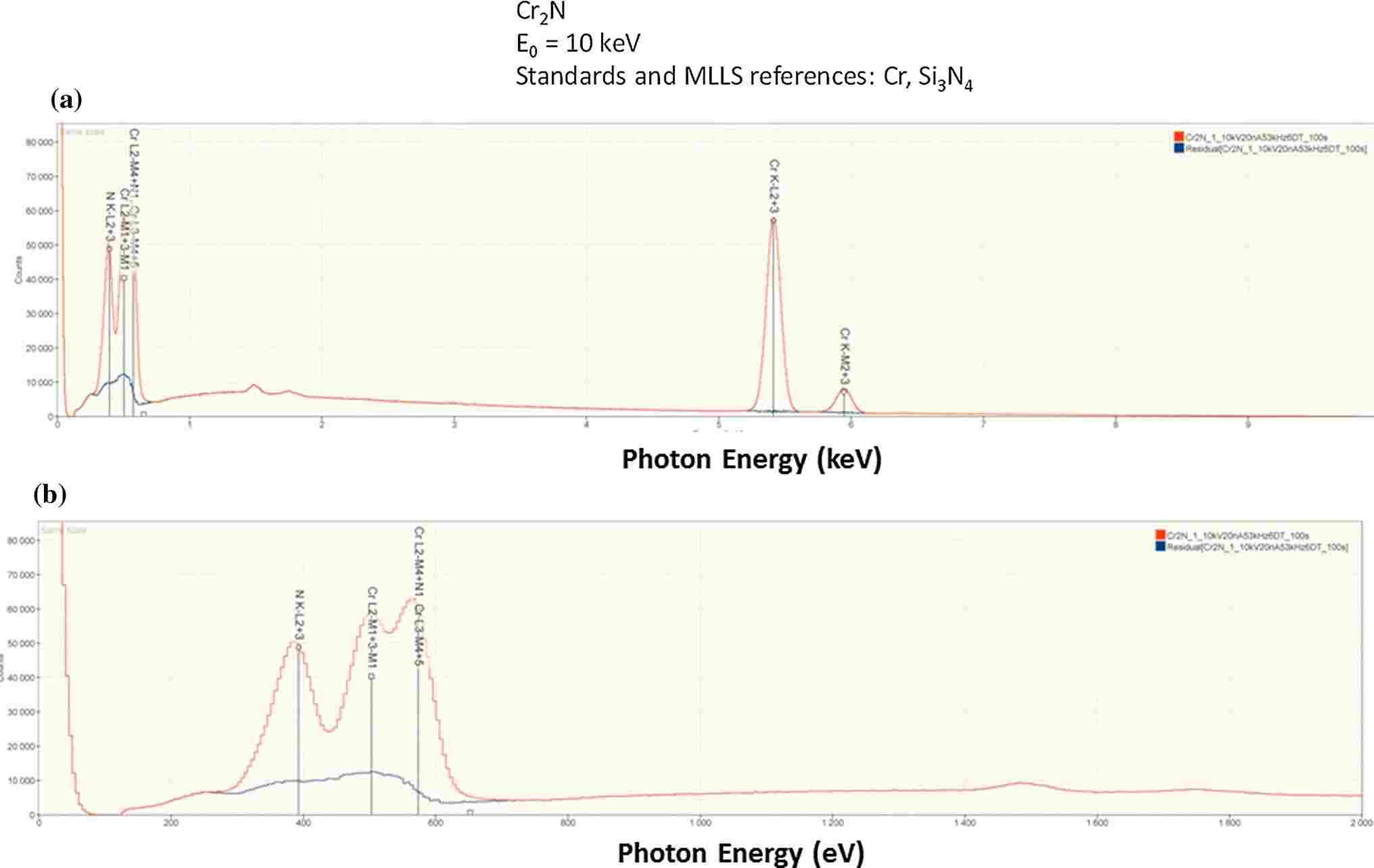
Figure 2. Full SDD-EDS spectrum of Cr₂N at 10 keV, the enlarged low-energy region, and the residual spectrum after multiple linear least-squares fitting. DOI: 10.1007/s10853-014-8685-2
The method carries a hidden assumption: that a given line has the same shape in the reference and in the unknown. Light elements break it routinely. Their K lines come from valence electrons filling a 1s vacancy, so any change in bonding reshapes the valence states and moves both peak position and peak profile.
Soft X-ray emission spectroscopy measures the shifts directly. Elemental boron sits at 183.5 eV; B₄C moves to about 184 eV and loses intensity on the low-energy side; FeB and Fe₂B grow a shoulder near 187 eV; B₂O₃ shifts down to 180.5 eV with two satellites alongside.
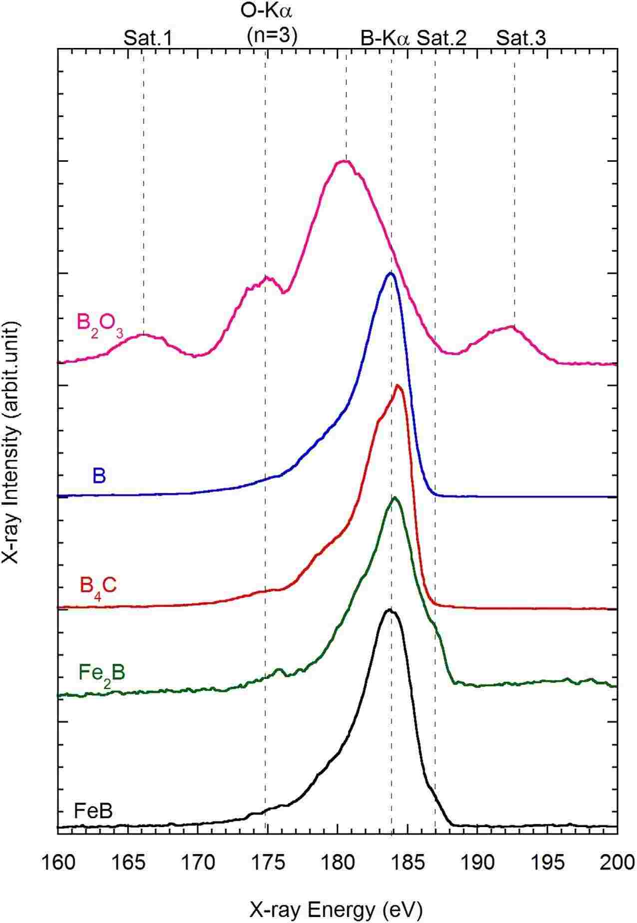
Figure 3. B-Kα spectra of B₂O₃, B, B₄C, Fe₂B and FeB measured by soft X-ray emission spectroscopy. DOI: 10.1038/srep25700
A few eV is nothing against the resolution of EDS, so the EDS spectrum shows a single broad lump either way — but the difference in shape is still in there.
And it ends up in the residual. When reference and unknown differ in chemical state, the mismatch survives the fit and distorts the net intensity that is extracted; NIST, examining residuals at 5 keV, listed the bonding-induced energy shift among the contributing factors.
Peak shape is not the only intrusion. Some of the signal does not come from the bulk at all. The beam cracks hydrocarbons adsorbed on the surface and left in the vacuum, laying down carbon exactly where it is looking — the longer it dwells, the thicker the layer — and air exposure adds oxide or sulphide on top. Lower the voltage and the excitation volume shrinks towards the surface, so the surface's share of the signal grows.
NIST saw exactly this in AlN. Measured at 15, 10 and 5 keV and normalized on N Kα, the C and O signals climbed steadily as the voltage dropped, and the sample was dropped from the accuracy statistics as a result.
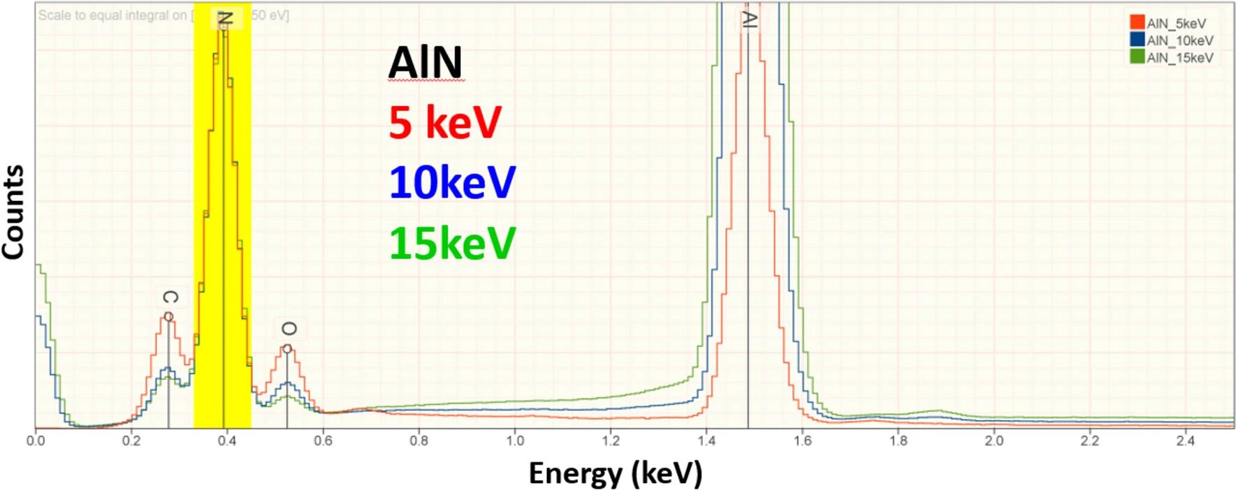
Figure 4. EDS spectra of AlN at 15, 10 and 5 keV, each normalized to the N K peak intensity. DOI: 10.1007/s10853-024-10285-4
Insulators are usually coated with 8–10 nm of carbon to stop charging, and that film both emits C and absorbs low-energy photons. Above 10 keV the effect on accuracy is negligible; below 5 keV, a mismatch in coating thickness between sample and standard becomes a real error. The raw totals NIST obtained at 5 keV spread from 0.8 to 1.2, which the authors put down mainly to coating differences.
Lithium by difference inherits every one of these errors. One cathode study assigned whatever mass fraction was missing from the un-normalized total to lithium: uncoated samples gave 6.0–6.4 wt%, close to the 6.4 wt% expected for the fully lithiated state after the first formation cycle, while gold- and carbon-coated samples gave 10.6 and 10.4 wt%.
Coating, surface layer and self-absorption all scale with voltage. Electron range goes roughly as E₀1.66, so dropping to 5 keV generates the X-rays nearer the surface and shortens the exit path; the photons are still low in energy, but the absorption correction has already shrunk appreciably.
The payoff is measurable. At 5 keV, NIST quantified 263 standard measurements across 39 elements in 113 materials: more than 98% of the results landed within ±5% relative deviation and 82% within ±2%, and results from 0–1.5 keV peaks distributed much as those from 1.5–5 keV peaks did.
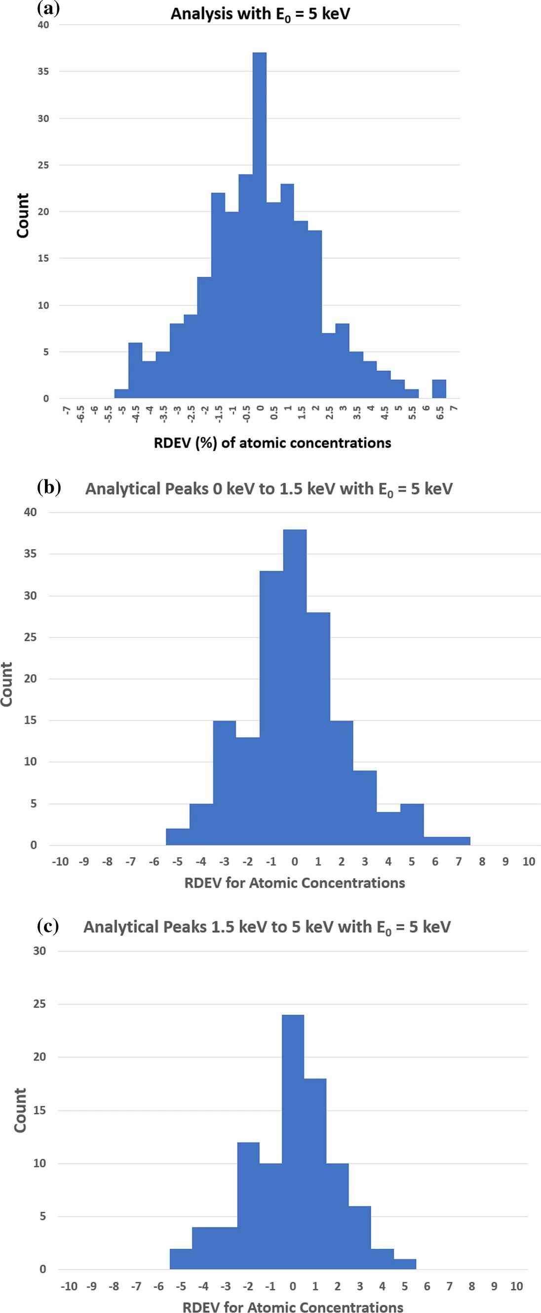
Figure 5. Distribution of relative deviations in atomic concentration from standard-based quantification at 5 keV: all results, 0–1.5 keV peaks and 1.5–5 keV peaks. DOI: 10.1007/s10853-024-10285-4
There is a limit to how far this can be pushed. 5 keV is the lowest voltage at which every element except H and He still has a usable line; further down, elements such as Ti and Ba have to be read from their low-energy L or M lines, which share the region with the light-element K lines.
Low voltage also means surface sensitivity, and that is a double-edged property. The 5 keV statistics excluded samples with very thick surface layers, for good reason: once an oxide or sulphide layer occupies a serious fraction of the electron range, the excitation volume holds two materials at once and the uniform-composition assumption behind k-ratio quantification no longer holds.
The practical test is a voltage series. Step from 10 keV and above down through 5 keV and watch the C and O peaks against the rest of the spectrum; a surface layer comparable in thickness to the electron range will make itself known.
Voltage is one variable; the standard is the other, because it fixes the scale on which net intensity becomes concentration. Standards-free quantification substitutes calculated or database intensities for measured ones, and those calculations lean on atomic parameters — fluorescence yields, mass absorption coefficients — that are known only to modest accuracy. One 2013 commercial standards-free package, assessed by NIST, needed a window of about ±30% to capture 95% of results.
Measured standards do considerably better. With pure elements or stoichiometric compounds, and k-ratios taken at 10 keV, about 10% dead time and roughly 10⁷ counts per spectrum, C, N, O and F come out within about ±5% — enough to tell Cr₃C₂ from Cr₇C₃ from Cr₂₃C₆, or SiO₂ from SiO, or CuO from Cu₂O. In thoroughly oxidized systems such as ceramics, glasses and minerals, oxygen is often calculated from the cation valences instead.
That calculation needs the valences to be known, and it offers no spatial information. Where the light-element distribution has to be mapped at the nanometre scale, a signal that never involves X-ray emission is the better bet. EELS records the energy lost by transmitted electrons as they excite inner shells; fluorescence yield does not enter, and detection limits reach 0.005–0.1 at%.
Applied to the same Cr₂N precipitate, EELS returned both the Cr- and the N-depleted zones, of equal width at about 70–100 nm, in agreement with the denoised STEM-EDS maps.
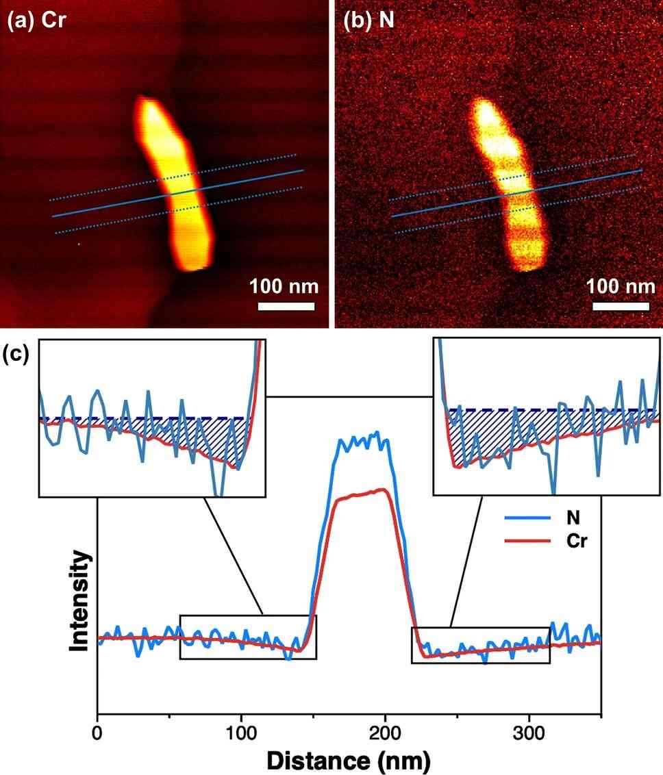
Figure 6. Cr and N EELS elemental maps of the Cr₂N precipitate and intensity profiles across the precipitate. DOI: 10.1038/s41598-020-70674-y
The costs are real: the foil has to be thin, the multiple-scattering background has to be stripped out — with some risk of distorting the spectrum — and the measurement is slower and more expensive than EDS.
Nor does EELS deliver chemical state. Boron speciation demands an energy resolution that neither EDS nor WDS can reach, which is where a soft X-ray emission spectrometer on an electron microprobe comes in: an aberration-corrected grating with parallel CCD detection records the spectra, and the B Kα profile separates the residual B₄C particles from the iron boride regions in control rods after oxidation testing.
SAT NANO specializes in the development, production, and application of nanomaterials. Its portfolio covers carbon nanomaterials (graphene, carbon nanotubes, nanocellulose), metal powder ,alloy powder, carbide powder, oxide powder, and emerging two-dimensional materials such as MXenes, serving plastics modification, coatings, energy, electronics, biomedical research, and new energy applications. If you have any enquiry, please feel free to contact us at sales03@satnano.com